Turbulence Modeling Deep-dive

A Turbulence Modeling Deep-dive with Azore CFD’s Lead Developer

By Dr. Jeff Franklin, P. E.

In today’s blog article, the lead developer of Azore, Dr. Jeff Franklin, P.E., explains the nuances of turbulence modeling and compares the k-ε and the k-ω SST turbulence models.

Azore’s latest release, Azore 2024R1, gives users incredible flexibility in turbulence modeling. Azore now integrates the k-ω SST turbulence model in addition to the widely used k-ε model. Along with this change, the wall function implementation smoothly accommodates variations in near wall mesh length scales of Y+ < 1 up through the fully turbulent Y+ length scales.

Read on to explore all things turbulence modeling with Dr. Franklin.

Does it matter what turbulence model you choose?

When working on a CFD project, you have many decisions to make about what to do to make the whole simulation and reporting process successful. The better decisions you make at the beginning of the process, the better outcome you will have further downstream. For example, the decisions you make about mesh topologies and boundary conditions all play a role in why you might choose a particular turbulence model and what you expect to get out of it. Since Azore now has both the k-ε and the k-ω SST models built into the solver, it’s worth it to dig into why you might choose one model over another, and to know the ramifications of the choices you make.

The k-ε model: simple and stable

Turbulence models in general can be thought of as the mother of all empirical relationships. These empirical estimations provide a bridge for a CFD tool to estimate the influences of turbulence without modeling the exact details for the turbulence physics that are impractical to include. The k-ε model is one of these empirical relationships that we use to represent turbulence in CFD tools. We know the fundamental equations for momentum, conservation of mass, conservation of energy, and conservation of species, but those equations don't really include turbulence unless you run them as highly detailed, transient simulations. Almost all real-world, flow problems are influenced by turbulence, so we need to include the impact of turbulence on the those equations in some way. The way we do that is with turbulent viscosity, which on a really basic level, helps us to “mix things up.” The turbulent viscosity is used in all of our conservation equations to represent turbulence, and in the k-ε model, it’s defined by this equation:

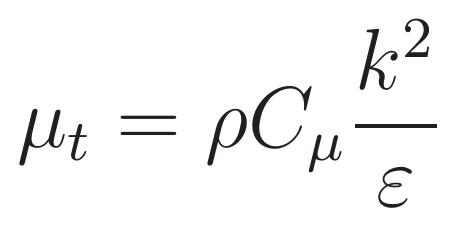
The Turbulent Viscosity Equation (k-ε Model)

As a two-equation turbulence model, the k-ε model relies on two fundamental relationships, the turbulent kinetic energy (k) and the dissipation rate (ε). The turbulent kinetic energy represents the local eddies, or the tumbling flow that's not resolved within the grid. The dissipation rate represents how quickly that turbulent kinetic energy dies, or dissipates. We essentially have one quantity that marks the generation of the turbulent kinetic energy and another that makes it disappear, and the ratio of these two values (k²/ε) helps quantify the local turbulence levels in the model.

The equation for turbulent kinetic energy is as follows:

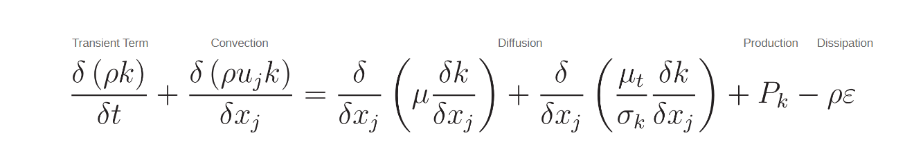
Turbulent Kinetic Energy Equation (k-ε Model)

The leftmost term is the transient term which says how turbulent kinetic energy changes with time, if we run a transient simulation. Next is the convective term: as your flow moves from one location to another, the turbulent kinetic energy travels with it. To the right is the diffusion of k, which shows how the value of k in one particular location affects neighboring locations. High energy and low energy areas will influence each other. The diffusion term also includes the effective turbulent viscosity (μ_t) along with a tuning constant (σ_k) another empirical parameter in the model. In Azore, the tuning constants are not accessible from the GUI since not many people change them. But if you want to, you can go into the input files and change them manually.

All of these terms so far characterize the transport of turbulent connected energy throughout the domain, but the next term, P_k is the turbulence production rate, which describes the generation of turbulence. The production rate is defined by the following equation, depending primarily on the velocity gradients.

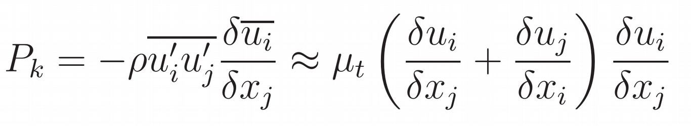
Turbulence Production Rate Equation (k-ε Model)

This dependence is important. How the velocity gradient is calculated can affect the turbulent production and ultimately the turbulent kinetic energy in the whole domain. If you have an algorithm that has very smooth calculations of gradients and they result in very stable numerical behavior, then you're going to get a very low value or gradient, and the turbulent production term is going to be smaller. If the algorithm tries to capture local gradients very sharply, and captures the gradients very well, then you’ll tend to get higher values for these gradients, which in turn will have an impact on the turbulent production rate.

This is simply an effect of the discretion scheme that the algorithm itself uses. One of the reasons you can see such a large difference in the implementation of a particular turbulence model from one code to another comes down to how the turbulent production rate is calculated. How and why gradients are used is especially important when it comes to comparing the k-ε and the k-ω SST models, because the k-ω SST model uses gradients heavily.

The last term in the equation ( – ρε) quantifies the decrease in turbulent kinetic energy due to the dissipation rate (ε), which is scaled by the density of the fluid. The following equation governs the dissipation rate:

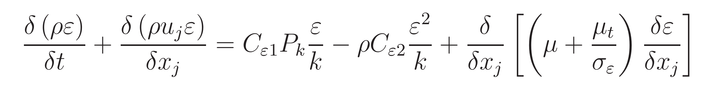
Dissipation Rate Equation (k-ε Model)

This equation doesn't have as much of a physical relationship, but depends mostly on length scale, which we know from the boundary conditions we put into the model. Usually the dissipation rate is characterized by some kind of length scale such as a hydraulic diameter. This makes sense because an eddy can only get so big, and its size is somewhat controlled by the geometry of the system. Generally speaking, if a pipe has a hydraulic diameter of one, then you would expect that the eddy can get no larger than one. The equation for dissipation rate contains some constants (C_ε1, C_ε2)and also the production rate. The ratio of the first two terms on the right side of the equation is what mostly controls how this field evolves in a simulation.

The standard k-ε turbulence model is a simple model. It's been around for years and years, but it works quite well. One of the reasons it works so well is because of its simplicity, which gives it strong numerical stability.

The k-ω SST model: blending and bounding

The k-ω SST turbulence model is a blend of two turbulence models, the k-ε model and the k-ω model. It was originally proposed by Dr. Florian Menter, who noted that the k-ω model has powerful numerical properties right near solid walls. This is very desirable because a lot of the flow structures that frame CFD problems happen to be near the wall and so we want to get that right. The problem with k-ω is that it does not do a good job in the far stream and has numerical issues, particularly with dissipation. Conversely, the k-ε model is known to have more difficulty near the wall, due to the way ε is characterized as it approaches the wall. But unlike the k-ω model, it does a really good job in the bulk flow.

What Menter tried to achieve is a combination of the two turbulence models, capturing the strengths of both. To accomplish this blending, the combined model uses many heuristics to bound the turbulent flow variables by expected behavior. It’s well-documented that the k-ε model can at times violate the expected values of the turbulent kinetic energy, and that’s not desirable. The idea is to keep those violations in check and keep all of the values reasonable. That is why the k-ω SST turbulence model uses bounding or heuristics to sort of “crop” the solution in these areas. The advantage of this is that it keeps things bounded, but the disadvantage is that it leads to numerical instability. Anything that has an “if statement” or truncation in it makes it much more challenging to solve numerically.

The k-ω SST model appears very similar to the k-ε model, but the details are significantly different in how the terms of the governing equations are put together. The turbulent viscosity is similar to the k-ε model, except that in the denominator it contains a limiting function.

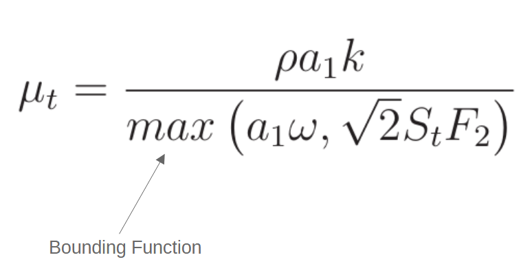
Turbulent Viscosity Equation (k-ω SST Model)

This max function is just one example of bounding that takes place within the k-ω SST model. If you use the left hand value in the max function, you essentially get the standard k-ε relationship for turbulent viscosity using the relationship between ω and ε, which is ε = β^*kω = C_μkω. The right value of the max function contains additional limiters and introduces dependence on the velocity gradients.

We should consider the impact of this on our model. The gradient dependency means that poor quality cells where you might have anomalous velocities will all of a sudden impact the turbulent viscosity in a spot wise way. So any low mesh quality that you might have in your model is going to become more sensitive because of these relationships.

The turbulent viscosity is used in the primary variables according to the following three relationships: the effective viscosity, the effective thermal conductivity, and the effective diffusivity.

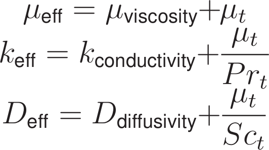
Substitutions made to primary variables

These relationships introduce two new empirical constants into the model, namely the turbulent Prandtl number and the turbulent Schmidt number.

The equation for the turbulent kinetic energy in the k-ω SST model is as follows:

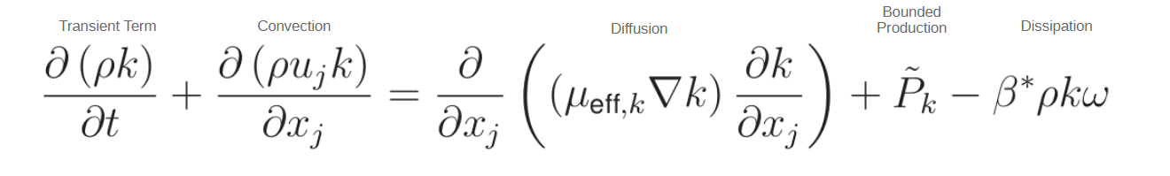
Turbulent Kinetic Energy Equation (k-ω SST Model)

The terms in this equation are similar to those in the k-ε model, but a few of the key variables are defined by blended relationships. For example, the μ_eff,k is defined by the turbulent viscosity, in addition to the function below, on the right. This is where the blending of the two turbulence models comes into play, with essentially a σ_k1 value that corresponds to the k-ε model and a σ_k2 value that corresponds to the k-ω model.

This blending function enables the turbulent kinetic energy equation to look like either the k-ε or k-ω version of the model depending on the distance away from the wall. Another difference is that instead of using the production rate as-is, the k-ω SST model uses an empirical relationship for the production rate that introduces another limiting function into the model.

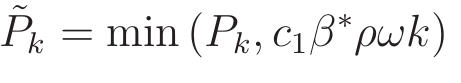
This additional truncation is essentially bounding the turbulent kinetic energy to keep it in a range that seems to be more reasonable. 

The equation for the turbulence dissipation utilizes a blending function similar to the one used in the turbulent kinetic energy equation:

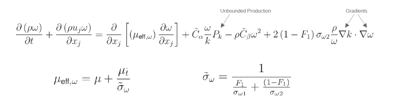
Turbulent Dissipation Equation (k-ω SST Model)

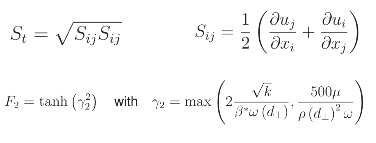
The equation for turbulence dissipation notably includes a gradient of the turbulent kinetic energy in the ω term along with a gradient of the variable itself. The internal solver mechanisms of how these gradients are calculated can have a big impact on the value of ω. The blending function below involves a cascade of choices that have been made in order to bound this value.

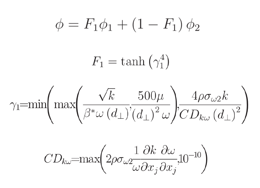
Blending Function

In the blending function, F₁ is a hyperbolic tangent of γ₁, which depends on several other variables – the turbulent kinetic energy, the dissipation rate, and the distance from the nearest wall (d_┴). The constant CD_kω is also dependent on the gradient of the variables we are trying to solve, which complicates things numerically. The F₁ variable is bound by multiple limiting functions. Whether or not this CD_kω equation is activated becomes highly dependent on the implementation of the gradients and whether they're large or small. Even simulation choices can also play a role in this, such as running with single or double precision.

In Azore, when you have the k-ω SST model enabled, there will be an additional field – the wall distance (d_┴). The image below shows this field, and the k-ω SST model equations blend together to apply the k-ω relationships near the wall and the k-ε relationships in the bulk flow.

Wall Distance Field in Azore

The challenge with the k-ω SST model continues to be its stability, or ability to converge. Instability is inherent to the model design, coming from the built-in limiters and bounding functions. One feature available in Azore is the ability to easily switch between the two turbulence models. If using the k-ω SST model is causing a lot of instability, it can help to start off by using the k-ε model. At any point during a run you can switch the turbulence model, and the good news is that Azore will automatically convert the ε values into ω values.

Which model should you use? It depends.

When it comes to simulation choices in CFD, there are very few absolutes. More often than not, we see very similar solutions between the k-ω SST and the k-ε method when a CFD model converges. When you get into more complex industrial systems, chances are, if the problem is not well-posed, the k-ω SST model may be unsteady. To evaluate the results from such a simulation, some kind of averaging will be used, which nominally may end up very similar to the k-ε results. The k-ε turbulence model will give you a more dispersed solution in general, since it is more stable and does a lot more averaging.

The “best” turbulent model depends on the geometry of the system and the design goals of the simulation. The k-ω SST model may be preferable for problems where the wall treatment is particularly important, such as skin friction problems or cases of flow-induced separation. If the design criterion lies in a plane near to some predicted flow separation, then the turbulence model you use might be more significant. But if the goal plane is farther downstream, using a more complex turbulence model is only adding time and cost to your CFD process. Prior to any simulation, we ought to consider the physics and geometry, always with the design goals in mind.

Fluid Dynamics Discussions with Azore CFD on YouTube: Explanation of the k-epsilon Turbulence Equations with Dr. Jeff Franklin