Case Study: Power Plant Ductwork
By Dr. Jeffrey Franklin, P.E.
Analysis of the velocity profiles and pressure losses within the ducting system
Introduction
The inception of an engineering simulation effort begins by identifying some key objectives. Once the simulation objectives have been determined, it is important to match these objectives with the proper simulation tools. Computer aided engineering (CAE) is a common practice in this high tech age, and there are a wide array tools available for performing numerical analysis. Choosing the right simulation tool for a particular objective is an important step toward a successful simulation effort. To make this choice, identify the necessary physics and the numerical techniques that are required to meet the objectives of the modeling effort. Once these choices have been made, a software tool that includes the physics and numerical methods can be chosen. Many times, there are a number of software choices available that provide the necessary features for a given simulation objective. The question then is, which software tool should be used? If the physics and the numerical techniques are the same for two different software packages, will the predictions of the simulation tools be the same? If there are differences, would the differences be enough to impact engineering choices that are being made based on the simulation predictions?
Case Study
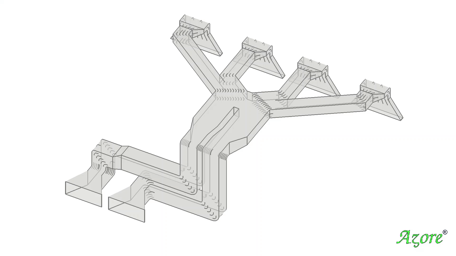
The system being analyzed is a typical representation of a ducting system located between the boiler and the pollution control equipment for a larger size power plant. The length scale for this geometry is fairly large with the duct cross sections having dimensions on the order of 20 - 30 ft (6 - 10 meters). This duct geometry includes a number of bends with flow control devices and two separate ducting systems that combine into one common system and then divides again into separate ducts.
Objectives
The objectives of the simulation effort will be limited to characterizing the gas velocity, temperature, and pressure patterns within the section of duct system selected. Since the flow rate through the system is typically constant at a particular operating condition, we will focus our analysis to a steady state flow condition. From an engineering perspective, the simulation predictions should help evaluate the velocity profiles and pressure losses within the ducting systems, providing insight into the optimal design of both the duct routing and internal flow control devices.
Physics and Numerical Methods
Since the focus of this discussion is centered around the application of CAE tools and in particular computational fluid dynamics (CFD), the selected physics and numerical methods will be taken from this field. For the physics of the system, we will choose the Navier-Stokes equations to represent the fluid motion and the standard K-epsilon turbulence model for representing the small scale transient turbulent motion. The temperature of the gas stream will be assumed to be constant leading to constant fluid properties such as fluid density and laminar viscosity. The control volume method has been selected for approximating the differential equations (the most widely used numerical technique in CFD).
Software Selection
Two CFD software packages have been selected for simulating the ducting system: Azore® and ANSYS® Fluent®. For the purposes of comparison, a single mesh topology was selected consisting of ~1.4 million computational cells. Mesh topology featured primarily polyhedral and hexahedral cells, with some tetrahedral cells in the more complicated regions. Each software package provides a framework for solving the Navier-Stokes and turbulence equations using the colocated control volume technique. An attempt was made to set the numerical solution parameters the same between the two software tools. Settings such as up-winding schemes, gradient calculations, and relaxation factors were all set the same between the two software packages.
Review of Results
To compare the simulation predictions between these two software packages, a number of solution cutting planes have been selected throughout the ducting system. Figures 1-8 detail the simulation predictions for each cutting plane selected. Each figure shows a wire frame of the ducting model with the relative location of the cutting plane location, along with the simulation predictions by both software packages positioned next to one another for comparison. The final part of this study is to review these simulation results and consider how any difference might impact engineering decisions that might be made based on these predictions. This exercise is left to the reader.
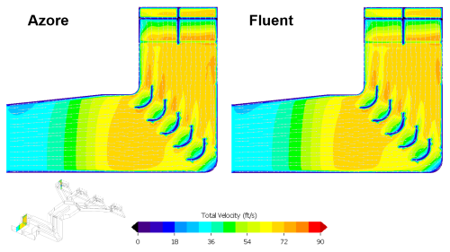
Figure 1
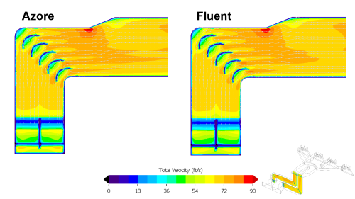
Figure 2
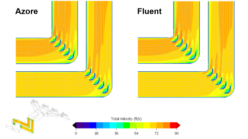
Figure 3
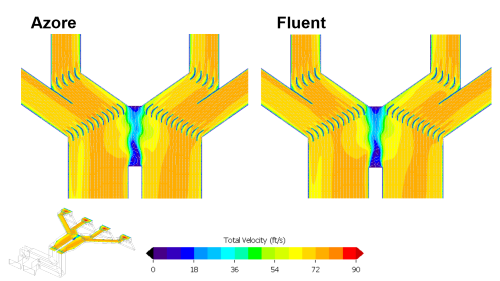
Figure 4

Figure 5
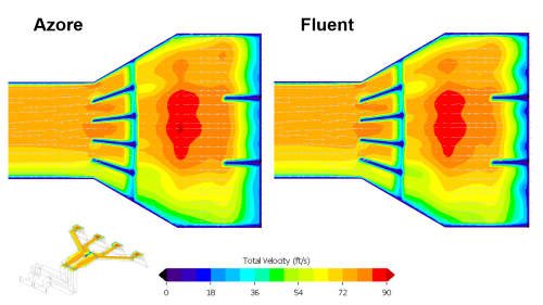
Figure 6
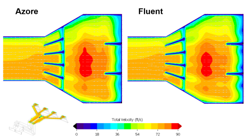
Figure 7
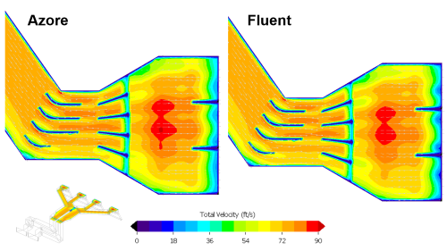
Figure 8
ANSYS® Fluent® is a registered trademark of ANSYS® Inc. and is not affiliated in anyway with Azore® Software, LLC.
Additional case studies can be found here.